What Does Expected Goals (xG) Actually Measure — And Why Most Fans Misunderstand It
The Problem xG Was Built to Solve
Before xG existed, the most common way to measure a team’s attacking performance was shots on target. It was a reasonable proxy. Teams with more shots on target generally won more matches. But it had an obvious flaw: it treated every shot as equal.
A shot from six yards out with the goalkeeper beaten is not the same as a shot from twenty-five yards into a crowd of defenders. Both count as one shot on target. Neither the stat sheet nor the post-match summary could tell you which team had actually created the better chances. xG was built specifically to solve this problem.
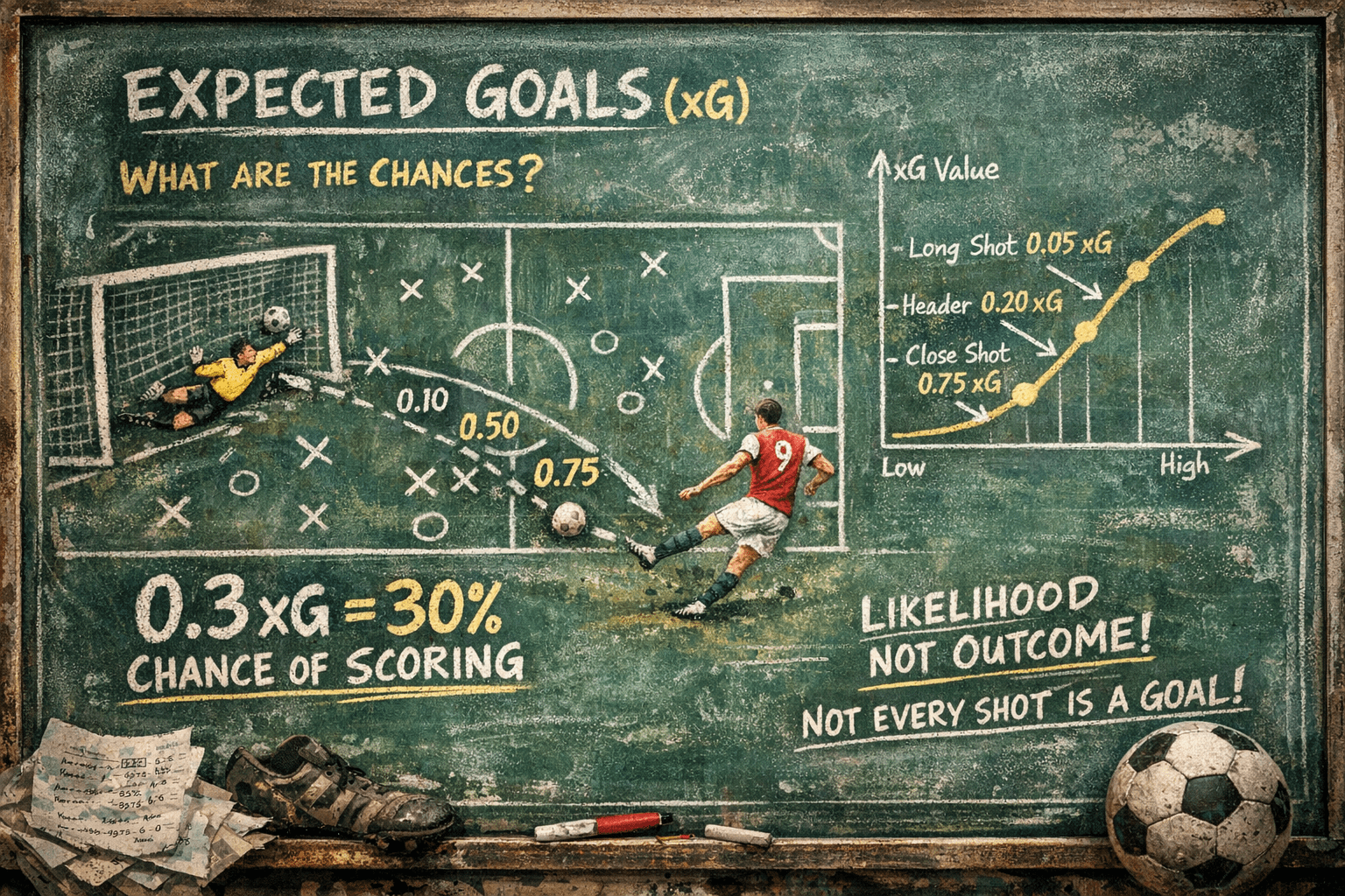
The underlying question is straightforward: given everything we know about a shot at the moment it is taken, how likely is it to result in a goal? The answer is expressed as a probability between 0 and 1. A shot assigned 0.10 xG would be expected to be scored once in every ten attempts, historically, from similar positions under similar conditions.
Where the Metric Came From
The history of expected goals is more complicated than most accounts suggest. The term “expected goals” appeared as early as 1993, in an academic paper by Vic Barnett and Sarah Hilditch examining how artificial pitches affected goal-scoring rates in English football. Their model was rudimentary and focused on broader game patterns rather than individual shots.
A more direct ancestor was a 1997 paper by Richard Pollard and Charles Reep titled “Measuring the Effectiveness of Playing Strategies at Soccer,” which calculated weighted shot values based on distance from goal, angle, whether the shot was headed, and defensive pressure. This was xG in structure if not yet in name.
The metric entered football’s mainstream in April 2012, when Sam Green, an analyst at OptaPro, published a blog post asking how to quantify which areas of the pitch were most likely to produce goals. Green proposed a model that calculated the probability of each shot being scored. He gave each shot a value he called an “expected goal.” The abbreviation xG followed.
“Green does not regard himself as the inventor of Expected Goals. But he was in the right place at the right time to give football what would turn out to be its breakthrough metric.” — Rory Smith, writing on the history of football analytics
The metric spread through analyst blogs and Twitter in the years that followed. Its moment of mainstream arrival came in November 2017, when Arsene Wenger discussed an Arsenal loss to Manchester City using xG figures. He was among the first high-profile managers to reference the stat publicly. By 2017, Opta had made it an official metric. Today it appears on Match of the Day, Sky Sports, and virtually every major broadcast.
How xG Models Actually Work
There is no single universal xG model. Different data companies produce different xG figures for the same shots. Opta’s model, one of the most widely used, is built on close to one million shots from forty competitions spanning 2018 to 2022. It uses a machine learning method called XGBoost to calculate shot probabilities from more than twenty variables recorded at the moment of the shot.
Angle to goal (central shots score more often than wide angles)
Goalkeeper position (how well placed is the goalkeeper to save?)
Body part used (foot or head, and which foot)
Type of assist (cross, through ball, cut-back, corner)
Match situation (open play, counter-attack, set piece, free kick)
Whether it was a rebound
Whether it came after a take-on
Whether it was a one-on-one situation
Penalties are given a fixed xG value of 0.79, reflecting their historical conversion rate across professional football.
The model does not measure what happens after the shot. It does not know whether the goalkeeper dived the right way, whether the ball hit the post, or whether the striker’s technique was good or poor. It only uses pre-shot information to estimate the probability based on historical precedent from similar situations.
This is a crucial distinction. xG is a measure of chance quality, not finishing quality. A striker who consistently scores chances with 0.10 xG is either finishing exceptionally well or getting lucky. Over a large enough sample, the data can begin to distinguish between the two.
Reading xG Correctly: Three Real Examples
In April 2025, Nottingham Forest beat Tottenham Hotspur 2-1. Tottenham had 22 shots and 6 on target. Their xG was 2.14. Forest had 4 shots, 3 on target, and an xG of 0.48. Forest won. The xG figures tell the accurate story: Tottenham created far more and far better chances but failed to convert them. Forest were clinical beyond what their chance quality suggested. Neither number alone tells you which team played better — together they do.
Cristiano Ronaldo went through a period at one stage of his career where his goal output dropped sharply and commentators suggested he had declined. His xG figures told a different story: he was continuing to get into excellent positions and generating high-quality chances. The model was right. He had not forgotten how to play. He was in a conversion slump, which corrected itself. This is exactly what xG is built for: separating genuine decline from statistical noise.
Arsenal in the early part of the 2022/23 Premier League season had a goal output that suggested they were a good team. Their xG figures suggested they were an exceptional one. The xG data indicated that their underlying chance creation was significantly stronger than their actual goals showed. Over the course of the season, their goal output converged toward their xG, and they finished second. The xG had been the more accurate predictor of quality all along.
xG Over Time: Why Sample Size Matters
This is where most fans misuse the metric. A team’s xG figures from a single match tell you relatively little. Football is a low-scoring, high-variance sport. Small samples produce misleading results. The research suggests the following rough guidelines:
| Number of Matches | Reliability of xG | How to Use It |
|---|---|---|
| 1 to 6 matches | Low | Context only. A single match xG figure can be dominated by chance events. |
| 7 to 16 matches | Growing | Patterns start to emerge. Worth comparing xG to actual goals to identify over or under-performance. |
| More than 16 matches | High | xG becomes a strong predictor of true team quality. Large persistent gaps between xG and goals deserve investigation. |
Research by analyst Ben Torvaney found that a ten-match rolling window is close to optimal for using xG to predict upcoming attacking and defensive performance. Below that window, noise drowns out the signal. Beyond a full season, actual goals become nearly as reliable as xG for assessing quality.
What xG Cannot Tell You
The metric has clear and honest limitations. Understanding them is just as important as understanding what the metric does well.
It ignores goalkeeper quality. A shot assigned 0.30 xG is estimated based on the average goalkeeper. An elite goalkeeper saving that chance routinely does not make the chance a lower xG opportunity. This is why some analysts use post-shot xG models that incorporate where in the goal the shot ended up, giving a better measure of goalkeeper performance than pre-shot xG alone.
It cannot measure off-ball movement. The run that creates space for a teammate does not appear in xG. The pressing trigger that forces a turnover in a dangerous position does not appear in xG. Much of what makes teams good is invisible to the metric.
Different providers produce different numbers. Opta, StatsBomb, and Understat all run different models with different input variables and training data. Their xG figures for the same shot are often not directly comparable. When reading xG statistics, it matters which model produced them.
It does not explain why things happen. A team with persistently low xG is not performing well in chance creation. xG tells you that. It does not tell you whether the problem is tactical, personnel-related, injury-driven, or systemic. Explanation requires video analysis alongside the data.
Teams that dominate territory get inflated xG. Paris Saint-Germain in Ligue 1 will always have a low opponents-xG figure partly because they spend so much time in the opposition half, creating more pressing opportunities regardless of actual pressing intent. Context is always required alongside the raw numbers.
xG and Goalkeepers: The Separate Problem
Expected goals has produced a useful secondary application in goalkeeper analysis. By comparing the xG of shots a goalkeeper faces against the goals they actually concede, analysts can measure whether a goalkeeper is saving shots they should save, conceding goals they should not, or performing broadly in line with expectations.
The metric Post-Shot xG (PSxG) goes further, incorporating information about where in the goal the shot ended up. A shot aimed at the top corner has a higher probability of scoring than a shot aimed at the centre of the goal from the same position. PSxG accounts for this, giving a better measure of shot quality that factors in the difficulty of the save.
In the 1993/94 Serie A season, AC Milan’s goalkeeper Sebastiano Rossi went 929 consecutive minutes without conceding a goal. Modern PSxG analysis applied retrospectively to that defensive record would almost certainly show he was facing low-quality chances, reflecting the defensive organisation in front of him. That is xG doing one of its most useful things: separating individual performance from the system supporting it.
Why xG Appears on Your TV and What That Means
The arrival of xG on broadcast television was not universally welcomed. Jeff Stelling, the Sky Sports presenter, made a pointed comment in 2017 after a match where a team with a better xG figure lost. His frustration was genuine and his point was not entirely wrong: in a single match, xG can feel disconnected from what the scoreboard says.
The critics have a point about single-match xG. Showing one match’s xG figure during a broadcast can mislead viewers into thinking the team with higher xG deserved to win. Whether they deserved to win is a philosophical question. Whether their chance quality was superior is what xG answers. Those are different questions.
Used correctly, broadcast xG adds something useful. It tells a viewer when a scoreline flatters or punishes a team relative to the quality of chances they created. Nottingham Forest beating Tottenham 2-1 with 0.48 xG to Tottenham’s 2.14 is genuinely informative. It does not mean Forest got lucky. It means they converted with exceptional efficiency and Tottenham did not. Over time, those two things tend to equalise. That is the core insight the metric offers.
xG in Club Operations: How Professional Teams Use It
The most sophisticated use of xG is not in broadcast graphics but inside clubs. Liverpool integrated xG into their analytical operations around 2012, under data scientist Ian Graham, who joined as Director of Research. The club used the metric to inform recruitment, tactical planning, and performance review. Their subsequent rise under Jurgen Klopp, while not solely data-driven, was built on a foundation that took analytical models seriously.
Modern clubs use xG as one input among many rather than a single answer. A scout identifying a striker will look at their goals minus their xG over multiple seasons. A striker who consistently scores more goals than their xG suggests is either a genuinely elite finisher or overperforming and likely to regress. A striker who consistently underperforms their xG may be a finishing problem, a system problem, or a statistical anomaly. The data narrows the field of investigation. It does not close it.
The Bottom Line
Expected goals is not a perfect metric. No metric is. It is, however, the most useful single number for evaluating attacking and defensive performance in football over a meaningful sample of matches. It measures something real: the quality of the chances a team creates and concedes, estimated from historical data on millions of similar situations.
Its limitations are worth knowing. A single match’s xG figure is noisy. The metric cannot see off-ball movement, pressing organisation, or goalkeeper positioning. Different providers produce different numbers. And it does not explain anything, only describe.
What it does well, it does better than almost anything else available. Over ten or more matches, a team’s xG figures tell you more about their underlying quality than the actual scorelines do. That is a significant thing to know about any metric. Most statistics in football cannot make that claim.